Why FLOPs mislead on real 3D hardware

FLOPs gets the ranking backwards

The metric most people use to estimate compute cost gets the ranking backwards on real hardware. FLOPs, a count of the arithmetic a network performs, said the dense voxel grid was cheap. Wall-clock time, the seconds you actually wait, said it was slowest by a factor of ten. Here is a case where the two measures disagree, the mechanism that explains the mismatch, and what it means for picking a 3D representation.

The experiment

ModelNet40, the standard benchmark of 12,311 CAD objects across 40 categories, was used. Every object was normalised to fit inside a unit sphere, then converted into four representations: point cloud (1,024 surface points), dense voxel grid (32×32×32 cube), sparse voxel (occupied cells only), and multi-view 2D (eight silhouettes). Each representation was trained on a small, deliberately old-fashioned network — PointNet for point-based inputs, VoxNet for 3D convolution, MultiViewCNN for 2D convolution — so the cost reflects the representation rather than a modern backbone.

Same objects, same train and test split, same 15 epochs, same batch size of 32, all on one passively-cooled Apple Silicon laptop. The processor is the built-in GPU with no fan. This is the kind of thermally constrained hardware a real robot or phone runs on, not the actively cooled card in a data centre. Only the representation varies.

Four ways to store one object

A 3D object on a computer is a surface floating in space. To feed it to a neural network you have to turn that surface into a grid of numbers. There is no single right way, and the choice you make quietly decides a lot about how fast the network runs.

Four ways dominate the field. I will describe them with the same object each time so the difference is visual, not abstract.

• Point cloud. Scatter a fixed number of dots on the surface, say a thousand, and store their coordinates. The network reads an unordered list of points. Cheap to store, but it throws away everything between the dots.
• Dense voxel grid. Divide the space around the object into a cube of smaller cubes, 32 along each edge, and mark each tiny cube as filled or empty. It is a 3D version of a pixel image. Complete, but for a typical object the vast majority of those cubes are empty air you still pay to carry around.
• Sparse voxel. Same idea as the dense grid, but store only the filled cubes and skip the air. This is the representation real lidar pipelines use, because the world is mostly empty and storing the emptiness is wasteful.
• Multi-view 2D. Stop trying to be three-dimensional. Take flat pictures of the object from several angles and let the network look at ordinary images. You lose depth, but you gain decades of optimisation built for photographs.

Here is the same aeroplane, four ways:

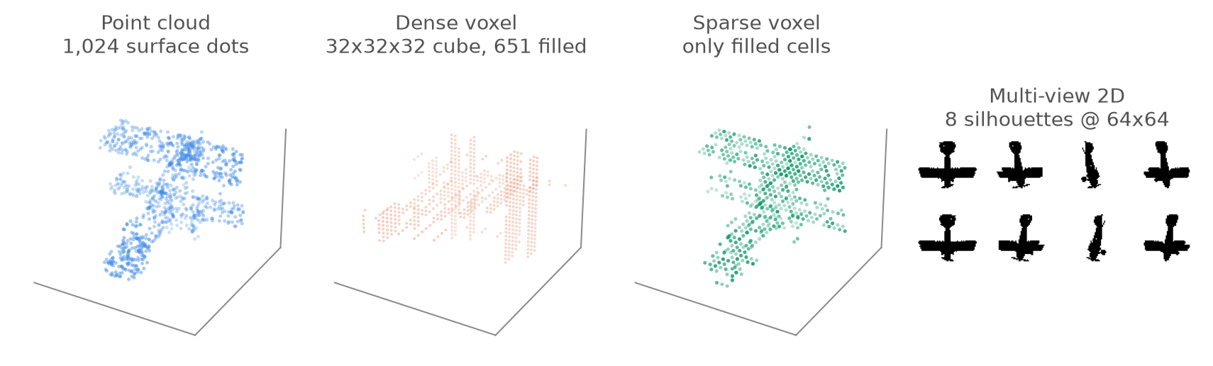
These are not four different objects. They are four different answers to the question "what numbers represent this shape", and each answer hands the network a different job.

The experiment

I took ModelNet40, the standard benchmark of 12,311 CAD objects across 40 categories. Every object gets normalised to fit inside a unit sphere, then converted into the four representations above. Each representation goes to a small, deliberately old-fashioned network: a PointNet for the point cloud, a VoxNet doing 3D convolutions for the dense grid, the same point-based net reading the sparse cells, and a small 2D-convolution net for the multi-view images. I chose old, simple networks on purpose, so the cost reflects the representation rather than some heavy modern backbone.

Same objects, same split, same 15 epochs of training, same batch size of 32, all on one passively-cooled Apple Silicon laptop. The processor is the laptop's built-in GPU with no fan. This is the kind of thermally constrained hardware a real robot or phone runs on, not the actively cooled card in a data centre.

The result: roughly a tenfold spread

Wall-clock time to train, 15 epochs, on that one laptop:

representation      train time   throughput   inference     accuracy   parameters
multi-view 2D         2.7 min     61.7 s/s    0.4 ms/sample   81.0%      1,149,000
sparse voxel         11.4 min     14.4 s/s    1.5 ms/sample   83.5%        815,336
point cloud          13.4 min     12.2 s/s    1.9 ms/sample   82.9%        815,336
dense voxel          29.2 min      5.6 s/s    3.4 ms/sample   84.9%        918,728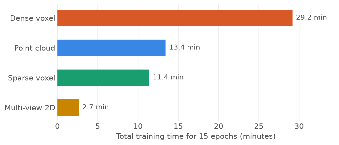

Throughput is samples per second — how many examples the network processes each second during training. It normalises for dataset size, so the ordering is more reproducible than total wall-clock alone. The same spread appears regardless of how many training examples you have. Multi-view 2D processes roughly 11 times more samples per second than the dense voxel grid.

Two things jump out before we get to the interesting part. The spread is large, roughly ten times from fastest to slowest. And the ranking is already not what model size would predict: the dense grid, which stores the most complete description of the shape, is also the slowest by a wide margin, while the multi-view pictures, which throw depth away entirely, are far and away the fastest.

FLOPs gets the ranking backwards

Here is where the theoretical measure breaks down. Look at the two charts below. They plot the same four representations, in the same colours, but the left chart ranks them by theoretical FLOPs and the right chart ranks them by the real wall-clock time measured above.

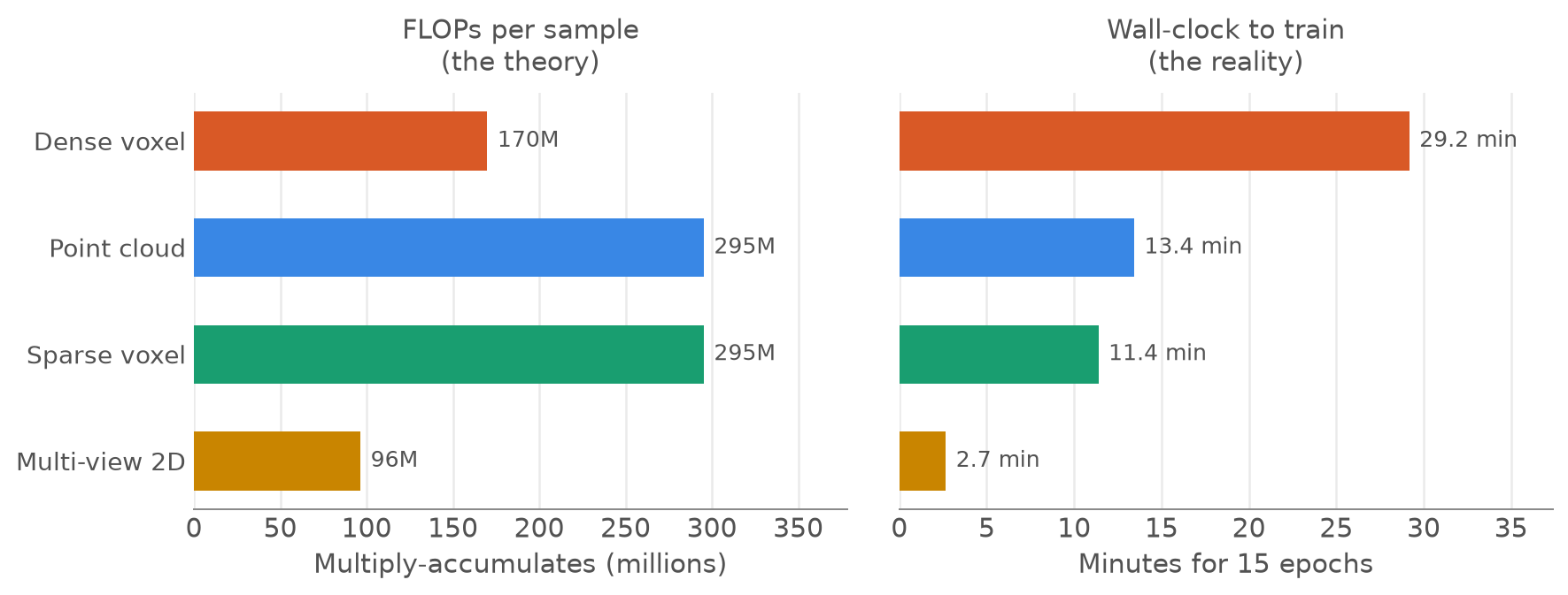
Read them together. On the left, the theory, the point cloud and sparse voxel come out most expensive at around 295 million operations each, the dense voxel sits comfortably cheap in third place at 170 million, and multi-view is the cheapest at 96 million. On the right, the reality, the dense voxel is the slowest of the four and multi-view is the fastest. The dense grid is the second cheapest by FLOPs and the most expensive by the clock. The two charts disagree, and that disagreement is the finding.

The parameter count tells the same story from another angle. The fastest model, multi-view, has the most parameters of the four. The slowest, dense voxel, is mid-pack on size. If you tried to estimate training cost from how big the model is, you would order them exactly wrong.

So what does predict speed, if neither size nor raw operation count does? It is how well the representation's compute maps onto the silicon. FLOPs assume two things that real hardware breaks. First, that every operation costs the same. Second, that operations can run back to back at peak speed. On a real chip neither holds. A 3D convolution sweeping through a dense cube spends much of its time fetching numbers out of memory, not doing arithmetic, and most of those numbers describe empty air. And the fast paths on the processor are tuned over many years for the dense 2D image workload that multi-view uses; the 3D cube is structurally similar but far less optimised. The representation's fit to the silicon dominates the operation count.

Dense representations cook themselves

Why does dense voxel throttle when multi-view does not? The answer is how the workload is structured. Dense 3D convolution is memory-bound: it moves a lot of empty air through memory for every useful arithmetic operation. That memory traffic generates heat, and the chip throttles itself to stay within safe thermal limits. Multi-view 2D, even with similar FLOPs, runs through well-optimised paths tuned for image workloads, which generate less heat per operation.

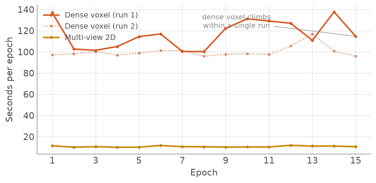
Run the dense model again from a cold start and you get a different total, because the workload reheats the chip during the run itself. Two clean runs of the same dense voxel model came in at 25.0 and 29.2 minutes, about fifteen percent apart. Cooling the machine down beforehand does not help. The heat builds up inside the run, not between runs.

This is what "fast" means on this class of hardware. The dense representation pays a super-linear penalty. More operations means more heat, which means more throttling, which means each batch takes longer, which extends the run, which generates more heat. The cost compounds. A benchmark run on a big, actively cooled data-centre GPU flattens this effect out of existence, because that chip never has to slow down. On the hardware a phone or a robot actually carries, the throttling is the cost.

What this does not prove

A few honest limits:

• One machine. The absolute numbers are specific to a passively-cooled laptop. On an actively cooled data-centre GPU the ranking could shift, and the throttling effect would largely vanish. The thermal finding is a property of edge-class hardware, not of the representations in general.
• Deliberately small, older models. I used PointNet and VoxNet on purpose so the cost reflects the representation rather than a modern backbone. The accuracy numbers sit below the state of the art, and the speed numbers would move with better nets. The relative ranking is the point, not the absolutes.
• The sparse column is a stand-in. Production sparse-voxel pipelines use a library called spconv for sparse 3D convolution, which I could not run on this hardware. I read the occupied cells as a point set through a PointNet instead, which tests the sparse-storage idea honestly but is not the production-grade net. Treat that column as indicative.
• One dataset, one task. ModelNet40 object classification, 15 epochs. A stronger claim needs more datasets, segmentation and detection tasks, and fully converged training.

The direction is real and the mechanism is real. The exact numbers are a snapshot of one laptop on two afternoons.

The practical takeaway

When you pick a 3D representation for something that runs on constrained hardware, treat it as an engineering decision, not a given. Three decision rules fall out of this:

• Before you trust FLOPs, ask: does this workload run on the hardware I will actually deploy on? If not, measure wall-clock and throughput. FLOPs alone got the ranking backwards here.
• Before you pick a dense 3D grid, ask: does the accuracy edge justify roughly an order of magnitude more wall-clock, plus the thermal tax that comes with it? If not, prefer multi-view 2D or sparse voxel.
• When you compare methods, use throughput, not total time — it normalises for dataset size and makes the ordering reproducible across experiments.

The fastest representation was the one that threw the most information away and asked the chip to do what it was already built for. That is not a coincidence. Fit to the silicon beats fidelity to the shape.

The code, the conversions, the timing harness, and the full numbers are on GitHub.

Further reading:

• Qi et al., PointNet (CVPR 2017), learning directly on raw point sets: arxiv.org/abs/1612.00593
• Su et al., Multi-View CNN for 3D Shape Recognition (ICCV 2015), rendering 3D shapes to 2D views for recognition: arxiv.org/abs/1505.00880
• Qi et al., Volumetric and Multi-View CNNs for Object Classification on 3D Data (ECCV 2016), the closest precedent, a controlled volumetric-versus-multi-view comparison: arxiv.org/abs/1604.03265
• Liu et al., Point-Voxel CNN (NeurIPS 2019), a hybrid that uses points for memory and voxels for convolution, evidence that no single pure representation wins: arxiv.org/abs/1907.03739